Tutorial
Parametric ANOVA with post hoc tests
Here is a simple example of the one-way analysis of variance (ANOVA) with post hoc tests used to compare sepal width means of three groups (three iris species) in iris dataset.
To begin, we will import the dataset using statsmodels get_rdataset() method.
>>> import statsmodels.api as sa
>>> import statsmodels.formula.api as sfa
>>> import scikit_posthocs as sp
>>> df = sa.datasets.get_rdataset('iris').data
>>> df.head()
   Sepal.Length  Sepal.Width  Petal.Length  Petal.Width Species
0           5.1          3.5           1.4          0.2  setosa
1           4.9          3.0           1.4          0.2  setosa
2           4.7          3.2           1.3          0.2  setosa
3           4.6          3.1           1.5          0.2  setosa
4           5.0          3.6           1.4          0.2  setosa
Now, we will build a model and run ANOVA using statsmodels ols() and anova_lm() methods. Columns Species and Sepal.Width contain independent (predictor) and dependent (response) variable values, correspondingly.
>>> lm = sfa.ols('Sepal.Width ~ C(Species)', data=df).fit()
>>> anova = sa.stats.anova_lm(lm)
>>> print(anova)
               df     sum_sq   mean_sq         F        PR(>F)
C(Species)    2.0  11.344933  5.672467  49.16004  4.492017e-17
Residual    147.0  16.962000  0.115388       NaN           NaN
The results tell us that there is a significant difference between groups means (p = 4.49e-17), but does not tell us the exact group pairs which are different in means. To obtain pairwise group differences, we will carry out a posteriori (post hoc) analysis using scikits-posthocs package. Student T test applied pairwisely gives us the following p values:
>>> sp.posthoc_ttest(df, val_col='Sepal.Width', group_col='Species', p_adjust='holm')
                  setosa    versicolor     virginica
setosa     -1.000000e+00  5.535780e-15  8.492711e-09
versicolor  5.535780e-15 -1.000000e+00  1.819100e-03
virginica   8.492711e-09  1.819100e-03 -1.000000e+00
Remember to use a FWER controlling procedure, such as Holm procedure, when making multiple comparisons. As seen from this table, significant differences in group means are obtained for all group pairs.
Non-parametric ANOVA with post hoc tests
If normality and other assumptions are violated, one can use a non-parametric Kruskal-Wallis H test (one-way non-parametric ANOVA) to test if samples came from the same distribution.
Let’s use the same dataset just to demonstrate the procedure. Kruskal-Wallis test is implemented in SciPy package. scipy.stats.kruskal method accepts array-like structures, but not DataFrames.
>>> import scipy.stats as ss
>>> import statsmodels.api as sa
>>> import scikit_posthocs as sp
>>> df = sa.datasets.get_rdataset('iris').data
>>> data = [df.loc[ids, 'Sepal.Width'].values for ids in df.groupby('Species').groups.values()]
data is a list of 1D arrays containing sepal width values, one array per each species. Now we can run Kruskal-Wallis analysis of variance.
>>> H, p = ss.kruskal(*data)
>>> p
1.5692820940316782e-14
P value tells us we may reject the null hypothesis that the population medians of all of the groups are equal. To learn what groups (species) differ in their medians we need to run post hoc tests. scikit-posthocs provides a lot of non-parametric tests mentioned above. Let’s choose Conover’s test.
>>> sp.posthoc_conover(df, val_col='Sepal.Width', group_col='Species', p_adjust = 'holm')
                  setosa    versicolor     virginica
setosa     -1.000000e+00  2.278515e-18  1.293888e-10
versicolor  2.278515e-18 -1.000000e+00  1.881294e-03
virginica   1.293888e-10  1.881294e-03 -1.000000e+00
Pairwise comparisons show that we may reject the null hypothesis (p < 0.01) for each pair of species and conclude that all groups (species) differ in their sepal widths.
Compact Letter Display
Post hoc test results can be condensed into a compact letter display (CLD), where groups sharing at least one letter are not significantly different from each other. This is useful for annotating plots or summarizing results in tables.
>>> x = [[1, 2, 1, 3, 1, 4], [12, 3, 11, 9, 3, 8, 1],
...      [10, 22, 12, 9, 8, 3], [14, 12, 16, 17, 5, 9]]
>>> pc = sp.posthoc_dunn(x, p_adjust='holm')
>>> sp.compact_letter_display(pc, alpha=0.05)
1    a
2    ab
3     b
4     b
Name: letters, dtype: object
Groups 1 and 2 share letter a (not significantly different), while groups
2, 3 and 4 share letter b (not significantly different). Group 1 is
significantly different from groups 3 and 4.
Block design
In block design case, we have a primary factor (e.g. treatment) and a blocking factor (e.g. age or gender). A blocking factor is also called a nuisance factor, and it is usually a source of variability that needs to be accounted for.
An example scenario is testing the effect of four fertilizers on crop yield in four cornfields. We can represent the results with a matrix in which rows correspond to the blocking factor (field) and columns correspond to the primary factor (yield).
The following dataset is artificial and created just for demonstration of the procedure:
>>> data = np.array([[ 8.82, 11.8 , 10.37, 12.08],
                     [ 8.92,  9.58, 10.59, 11.89],
                     [ 8.27, 11.46, 10.24, 11.6 ],
                     [ 8.83, 13.25,  8.33, 11.51]])
First, we need to perform an omnibus test — Friedman rank sum test. It is implemented in scipy.stats subpackage:
>>> import scipy.stats as ss
>>> ss.friedmanchisquare(*data.T)
FriedmanchisquareResult(statistic=8.700000000000003, pvalue=0.03355726870553798)
We can reject the null hypothesis that our treatments have the same distribution, because p value is less than 0.05. A number of post hoc tests are available in scikit-posthocs package for unreplicated block design data. In the following example, Nemenyi’s test is used:
>>> import scikit_posthocs as sp
>>> sp.posthoc_nemenyi_friedman(data)
          0         1         2         3
0 -1.000000  0.220908  0.823993  0.031375
1  0.220908 -1.000000  0.670273  0.823993
2  0.823993  0.670273 -1.000000  0.220908
3  0.031375  0.823993  0.220908 -1.000000
This function returns a DataFrame with p values obtained in pairwise comparisons between all treatments. One can also pass a DataFrame and specify the names of columns containing dependent variable values, blocking and primary factor values. The following code creates a DataFrame with the same data:
>>> data = pd.DataFrame.from_dict({'blocks': {0: 0, 1: 1, 2: 2, 3: 3, 4: 0, 5: 1, 6:
2, 7: 3, 8: 0, 9: 1, 10: 2, 11: 3, 12: 0, 13: 1, 14: 2, 15: 3}, 'groups': {0:
0, 1: 0, 2: 0, 3: 0, 4: 1, 5: 1, 6: 1, 7: 1, 8: 2, 9: 2, 10: 2, 11: 2, 12: 3,
13: 3, 14: 3, 15: 3}, 'y': {0: 8.82, 1: 8.92, 2: 8.27, 3: 8.83, 4: 11.8, 5:
9.58, 6: 11.46, 7: 13.25, 8: 10.37, 9: 10.59, 10: 10.24, 11: 8.33, 12: 12.08,
13: 11.89, 14: 11.6, 15: 11.51}})
>>> data
    blocks  groups      y
0        0       0   8.82
1        1       0   8.92
2        2       0   8.27
3        3       0   8.83
4        0       1  11.80
5        1       1   9.58
6        2       1  11.46
7        3       1  13.25
8        0       2  10.37
9        1       2  10.59
10       2       2  10.24
11       3       2   8.33
12       0       3  12.08
13       1       3  11.89
14       2       3  11.60
15       3       3  11.51
This is a melted and ready-to-use DataFrame. Do not forget to pass melted argument:
>>> sp.posthoc_nemenyi_friedman(data, y_col='y', block_col='blocks', group_col='groups', melted=True)
          0         1         2         3
0 -1.000000  0.220908  0.823993  0.031375
1  0.220908 -1.000000  0.670273  0.823993
2  0.823993  0.670273 -1.000000  0.220908
3  0.031375  0.823993  0.220908 -1.000000
Data types
Internally, scikit-posthocs uses NumPy ndarrays and pandas DataFrames to store and process data. Python lists, NumPy ndarrays, and pandas DataFrames are supported as input data types. Below are usage examples of various input data structures.
Lists and arrays
>>> x = [[1,2,1,3,1,4], [12,3,11,9,3,8,1], [10,22,12,9,8,3]]
>>> # or
>>> x = np.array([[1,2,1,3,1,4], [12,3,11,9,3,8,1], [10,22,12,9,8,3]])
>>> sp.posthoc_conover(x, p_adjust='holm')
          1         2         3
1 -1.000000  0.057606  0.007888
2  0.057606 -1.000000  0.215761
3  0.007888  0.215761 -1.000000
You can check how it is processed with a hidden function __convert_to_df():
>>> sp.__convert_to_df(x)
(    vals  groups
 0      1       1
 1      2       1
 2      1       1
 3      3       1
 4      1       1
 5      4       1
 6     12       2
 7      3       2
 8     11       2
 9      9       2
 10     3       2
 11     8       2
 12     1       2
 13    10       3
 14    22       3
 15    12       3
 16     9       3
 17     8       3
 18     3       3, 'vals', 'groups')
It returns a tuple of a DataFrame representation and names of the columns containing dependent (vals) and independent (groups) variable values.
Block design matrix passed as a NumPy ndarray is processed with a hidden __convert_to_block_df() function:
>>> data = np.array([[ 8.82, 11.8 , 10.37, 12.08],
                     [ 8.92,  9.58, 10.59, 11.89],
                     [ 8.27, 11.46, 10.24, 11.6 ],
                     [ 8.83, 13.25,  8.33, 11.51]])
>>> sp.__convert_to_block_df(data)
(    blocks groups      y
 0        0      0   8.82
 1        1      0   8.92
 2        2      0   8.27
 3        3      0   8.83
 4        0      1  11.80
 5        1      1   9.58
 6        2      1  11.46
 7        3      1  13.25
 8        0      2  10.37
 9        1      2  10.59
 10       2      2  10.24
 11       3      2   8.33
 12       0      3  12.08
 13       1      3  11.89
 14       2      3  11.60
 15       3      3  11.51, 'y', 'groups', 'blocks')
DataFrames
If you are using DataFrames, you need to pass column names containing variable values to a post hoc function:
>>> import statsmodels.api as sa
>>> import scikit_posthocs as sp
>>> df = sa.datasets.get_rdataset('iris').data
>>> sp.posthoc_conover(df, val_col='Sepal.Width', group_col='Species', p_adjust = 'holm')
val_col and group_col arguments specify the names of the columns containing dependent (response) and independent (grouping) variable values.
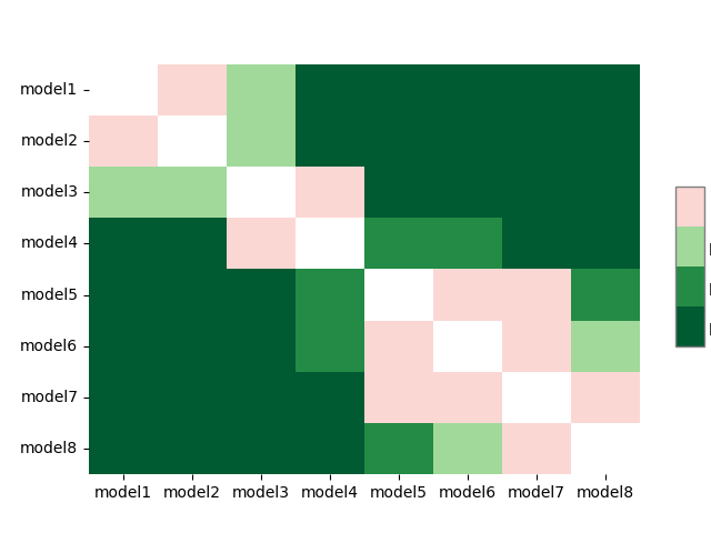
Significance plots
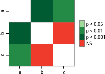
P values can be plotted using a heatmap:
pc = sp.posthoc_conover(x, val_col='values', group_col='groups')
heatmap_args = {'linewidths': 0.25, 'linecolor': '0.5', 'clip_on': False, 'square': True, 'cbar_ax_bbox': [0.80, 0.35, 0.04, 0.3]}
sp.sign_plot(pc, **heatmap_args)
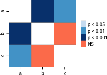
Custom colormap applied to a plot:
pc = sp.posthoc_conover(x, val_col='values', group_col='groups')
# Format: diagonal, non-significant, p<0.001, p<0.01, p<0.05
cmap = ['1', '#fb6a4a',  '#08306b',  '#4292c6', '#c6dbef']
heatmap_args = {'cmap': cmap, 'linewidths': 0.25, 'linecolor': '0.5', 'clip_on': False, 'square': True, 'cbar_ax_bbox': [0.80, 0.35, 0.04, 0.3]}
sp.sign_plot(pc, **heatmap_args)
Critical difference diagrams
Critical difference diagrams are another interesting way of visualizing post hoc test statistics. Firstly, in a block design scenario, the values within each block are ranked, and the average rank across all blocks for each treatment is plotted along the x axis. A crossbar is then drawn over each group of treatments that do not show a statistically significant difference among themselves.
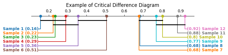
As an example, suppose we have a set of 8 treatments with 30 measurements (blocks) each, as simulated below. It could, for instance, represent scores for eight machine learning models in a 30-fold cross-validation setting.
>>> rng = np.random.default_rng(1)
>>> dict_data = {
    'model1': rng.normal(loc=0.2, scale=0.1, size=30),
    'model2': rng.normal(loc=0.2, scale=0.1, size=30),
    'model3': rng.normal(loc=0.4, scale=0.1, size=30),
    'model4': rng.normal(loc=0.5, scale=0.1, size=30),
    'model5': rng.normal(loc=0.7, scale=0.1, size=30),
    'model6': rng.normal(loc=0.7, scale=0.1, size=30),
    'model7': rng.normal(loc=0.8, scale=0.1, size=30),
    'model8': rng.normal(loc=0.9, scale=0.1, size=30),
}
>>> data = (
  pd.DataFrame(dict_data)
  .rename_axis('cv_fold')
  .melt(
      var_name='estimator',
      value_name='score',
      ignore_index=False,
  )
  .reset_index()
)
>>> data
      cv_fold  estimator     score
0          0      model1  0.234558
1          1      model1  0.282162
2          2      model1  0.233044
3          3      model1  0.069684
4          4      model1  0.290536
..       ...       ...       ...
235       25      model8  0.925956
236       26      model8  0.758762
237       27      model8  0.977032
238       28      model8  0.829890
239       29      model8  0.787381

[240 rows x 3 columns]
The average (percentile) ranks could be calculated as follows:
>>> avg_rank = data.groupby('cv_fold').score.rank(pct=True).groupby(data.estimator).mean()
>>> avg_rank

estimator
model1    0.208333
model2    0.191667
model3    0.366667
model4    0.495833
model5    0.708333
model6    0.737500
model7    0.850000
model8    0.941667
Name: score, dtype: float64
Again, the omnibus test result shows we can confidently reject the null hypothesis that all models come from the same distribution and proceed to the post hoc analysis.
>>> import scipy.stats as ss
>>> ss.friedmanchisquare(*dict_data.values())
FriedmanchisquareResult(statistic=186.9000000000001, pvalue=6.787361102785178e-37)
The results of a post hoc Conover test are collected:
>>> test_results = sp.posthoc_conover_friedman(
>>>     data,
>>>     melted=True,
>>>     block_col='cv_fold',
>>>     group_col='estimator',
>>>     y_col='score',
>>> )
>>> sp.sign_plot(test_results)
Finally, the average ranks and post hoc significance results can be passed to
the critical_difference_diagram() function to plot the diagram:
>>> plt.figure(figsize=(10, 2), dpi=100)
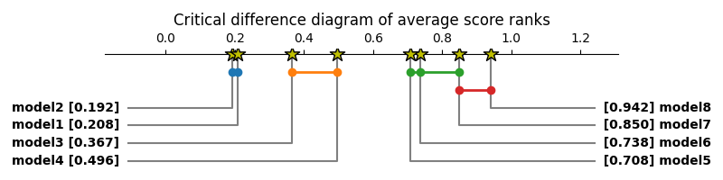
>>> plt.title('Critical difference diagram of average score ranks')
>>> sp.critical_difference_diagram(avg_rank, test_results)
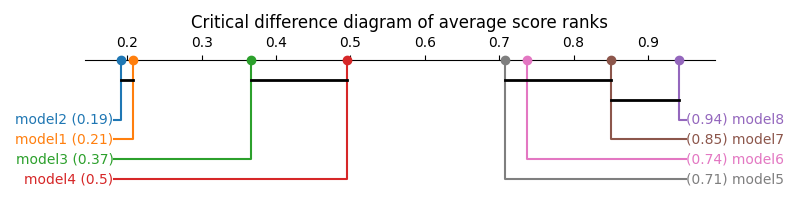
The diagram shows that model 8 is significantly better ranked than all models but model 7, that models 1 and 2 are worse than the others, and that 3 and 4 are also worse ranked than models 5, 6 and 7. Other comparisons, however, do not have sufficient statistical evidence to support them.
Several style customization options are available:
>>> plt.figure(figsize=(10, 2), dpi=100)
>>> plt.title('Critical difference diagram of average score ranks')
>>> sp.critical_difference_diagram(
>>>     ranks=avg_rank,
>>>     sig_matrix=test_results,
>>>     label_fmt_left='{label} [{rank:.3f}]  ',
>>>     label_fmt_right='  [{rank:.3f}] {label}',
>>>     text_h_margin=0.3,
>>>     label_props={'color': 'black', 'fontweight': 'bold'},
>>>     crossbar_props={'color': None, 'marker': 'o'},
>>>     marker_props={'marker': '*', 's': 150, 'color': 'y', 'edgecolor': 'k'},
>>>     elbow_props={'color': 'gray'},
>>> )